Smarter Task Estimating

In capital and IT projects, one bad estimate can derail millions in investments. Task durations are more than numbers—they’re predictions packed with risk. One misstep can trigger delays, balloon costs, or compromise quality. Traditional methods like PERT and triangular distributions often yield estimates that falter under scrutiny. This article offers a smarter path: a risk banding rubric to quantify uncertainty in clear terms, paired with beta distributions for high-confidence Monte Carlo simulations. By simplifying estimation and leveraging beta’s precision, we build schedules that stand up to reality.

The Estimating Trap: Why Traditional Methods Fail

Estimating task durations is a high-wire act with lopsided risks. Overestimate, and you get linear penalties—work expands to fill the time, per Parkinson’s Law, wasting resources and slowing progress. Underestimate, and nonlinear penalties hit hard: delays cascade across dependencies, defects pile up from rushed fixes, and high-risk shortcuts erode quality. A late task can derail an entire project, amplifying costs and stress. Projects are interconnected systems, so underestimation’s disruptions grow exponentially, making it the greater threat.

Human nature fuels this risk. We’re prone to optimism, assuming tasks will glide smoothly despite past hiccups. Buehler et al. (1994) call this the “planning fallacy,” where we fixate on best-case scenarios. Kahneman and Tversky (1979) note we ignore uncertainty ranges, favoring singular predictions. Flyvbjerg (2008) shows this optimism undercuts complex projects consistently.

PERT and triangular distributions don’t fix this. PERT’s 1:4:1 weighting of optimistic, likely, and pessimistic estimates assumes symmetry that real tasks rarely match. Triangular’s equal averaging oversimplifies variability. Both produce low-confidence estimates, vulnerable to nonlinear risks. Beta distributions, modeling skewed durations, counter optimism with higher confidence, protecting against surprises.

Risk Banding: A Practical Fix for Optimism Bias

Risk banding fights optimism with a rubric that sorts task uncertainty into intuitive levels, from “Minimal” to “Extreme.” It streamlines three-point estimating by linking optimistic, likely, and pessimistic durations to task traits like complexity or novelty. This curbs guesswork and feeds beta distributions for simulations, delivering schedules with greater confidence than PERT or triangular methods, safeguarding against underestimation’s chaos.

Inside the Rubric: 10 Levels of Uncertainty

Our 10-level rubric, inspired by Fibonacci-like growth, captures uncertainty’s non-linear escalation. The table below provides a range of uncertainty bands from Minimal to Extreme, a simple description to help humans decide which band a task belongs to, and lists the band Optimistic, Likely, and Pessimistic factors. It then calculates the beta parameters corresponding to those factors (computed per Davis, 2008):

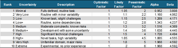
Duration and Confidence Level Calculations

With the factors and the Beta parameters we can now calculate durations and confidence levels for each band. Assuming a 10d task, let [a, m, b] be the Optimistic, Likely, and Pessimistic durations based on the rubric factors above:

• PERT: μ=(a+4m+b)/6, P% use Excel BETA.DIST(μ,alpha, beta, a, b)
• Triangular: μ=(a+m+b)/3, P% use Excel BETA.DIST(μ,alpha, beta, a, b)
• Beta: For p = 50% and p = 80%, use Excel BETAINV(p, alpha, beta, a, b)

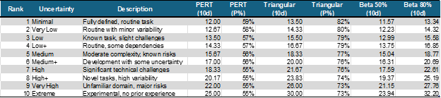
Scalability Note: Durations scale linearly with the base duration. For a 25-day task, multiply 10-day estimates by 2.5 (e.g., “High” PERT: 18.3 × 2.5 = 45.8; Beta 80%: 22.6 × 2.5 = 56.5). This ensures versatility for any task size.

Fast, Human-Friendly Estimating in Real Teams

Risk banding doesn’t just improve accuracy—it makes estimating and tracking progress faster and easier. Traditional three-point estimating asks engineers for optimistic, likely, and pessimistic durations, a process that feels tedious and abstract. With risk banding, you ask two simpler questions: “How long do you think this task should take?” and “What’s your level of uncertainty?” They provide a best-guess duration and pick a rubric level (e.g., “Medium” or “High”), which maps to precomputed factors. This cuts mental effort dramatically.

These subjective questions, framed in human-readable terms, align with how people think. Research backs this up: structured frameworks reduce cognitive load, making complex tasks feel intuitive (Sweller, 1988). Descriptive categories like “Low” or “Extreme” speed up decisions by tapping into familiar judgment patterns (Tversky & Kahneman, 1981). Simple heuristics, like choosing a rubric level, yield fast, reliable results under uncertainty (Gigerenzer & Gaissmaier, 2011). In practice, teams answer these questions in seconds, with less second-guessing.

For ongoing status collection, the rubric shines. Instead of revisiting three numbers, engineers update their best guess and uncertainty level as risks evolve—say, dropping from “High” to “Low+” after resolving a blocker. This streamlined process minimizes errors and keeps schedules current, freeing teams to focus on execution rather than paperwork.

What the Data Shows: Critical Path Impacts by Method

The image below shows a single critical path of 25 activities. The optimistic task duration and the risk band have been randomly generated for each task (save or open the image in a new tab to see full size):

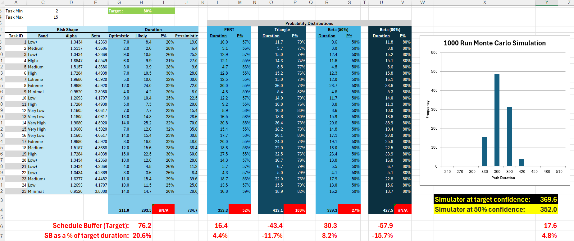
For each task, we can use our rubric to determine the following information:

• Likely duration, the probability of achieving the Likely duration, and the Pessimistic duration
• PERT duration and probability of achieving the PERT duration
• Triangular duration and probability of achieving the Triangular duration
• Durations based on the Beta Distribution 50% and 80% probabilities.

If we run a Monte Carlo simulation against this path we can compare the different deterministic path lengths with the simulated path. In this example, the Monte Carlo simulation showed that there is an 80% confidence the path will complete in under 370 days, and a 50% confidence that it will complete in under 352 days. Assuming we want to plan with 80% confidence, we can see that:

• If we use the Likely durations, the deterministic path will be 294 days. The Monte Carlo simulation shows there is zero chance of achieving that, so we will need to add 76 days of buffer to the schedule to reflect the inherent uncertainty.
• Using PERT durations, the path length will be 353 days. Monte Carlo shows that there is a 52% chance of hitting that number, and that we will need to add 16 days of buffer to protect our 80% plan.
• If we use Triangle estimates, the path length will be 413 days. This is 43 days longer than the 80% duration from the Monte Carlo simulation, and there is a nearly 100% chance we can hit this date.
• Beta 50% durations are similar to PERT in this rubric, but slightly more aggressive. The Beta 50 path is 339 days long with a 27% chance of being achieved, meaning we will need to add 30 days of buffer to protect the 80% confidence plan.
• Beta 80% durations are even more conservative than Triangle estimates. The Beta 80 path is 428 days long, which is 58 days longer than the 370 days we need for 80% confidence. None of the 1000 simulation runs ended up being that long, so again we have a very high confidence we can finish before 428 days have passed.

Which Duration Wins? A Scheduler’s Decision Guide

So, now we have five possible durations to choose from. Which one do we put in our schedules? If we make the tasks too long we run the risk of effort expanding to fill the time (Parkinsons Law), or procrastination leading to a rush at the end resulting in low quality and late delivery (Student Syndrome). If we make them too short we add a major non-linear risk of shortcuts in planning and design that drive increasingly high-risk practices and destructive late project dynamics (extra status meetings, cutting scope, defects, etc.) as teams try to "recover" when tasks start to slip.

In this example, we're going to pick the Beta 50 task durations with a 30-day buffer to protect the delivery. I think using PERT would also work well, but here is why Beta 50 is the best choice:

1. There is zero chance that the team will hit the mark using the Likely task durations. While we can add a 20% schedule buffer, setting impossible goals can be demoralizing to a team and should be avoided as that can lower performance.
2. The Beta 80 and Triangle estimates are too high, providing too much cushion in each task and driving the overall path duration higher than it needs to be. This excessive padding drives unnecessary cost into the plan.
3. The PERT estimates are achievable, allowing a greater than 50% chance of achieving each individual task within its planned duration, and needing only a 4% buffer to protect the target path duration of 370 days. That's not bad, but that buffer is a little bit skimpier than we would like for this example.
4. The Beta 50 gives the team a 50/50 chance of completing each task, and 30 days of buffer to use up if they start to get behind. This should keep everyone engaged, as with each task the team will see if they are gaining or losing buffer as they get closer to the finish.

The key insight here is that the way you plan drives real-world behaviors. Tracking buffer erosion against the time left to complete adds a competitive edge to the project that many teams find motivating. Setting impossible targets is demotivating, and to a lesser degree so is setting targets that are too easy to achieve. Finding the right balance can change from project to project and from team to team, but the way you build your plan will in all cases change how the team performs.

Final Thought: Plans Shape Performance

Optimism breeds underestimation—and with it, the chaos of delays, rework, and spiraling costs. Risk banding with beta distributions offers a sharper defense. By pairing structured uncertainty levels with powerful Monte Carlo simulations, we shift project planning from hopeful guesswork to high-confidence forecasting.

Our Fibonacci-inspired rubric simplifies estimates, streamlines status updates, and powers realistic schedules. And it scales: for smaller or more agile teams, a five-level version—Very Low (1.10, 1.30), Low (1.15, 1.45), Medium (1.30, 1.80), High (1.50, 2.20), and Very High (1.80, 2.80)—delivers the same rigor with less complexity.

Tailor the rubric to your team, your domain, your risk appetite. What matters most is this: the way you plan shapes how your team performs. Plans that ignore uncertainty erode trust and precision. But plans built on quantified risk unlock executional clarity—and often, a sense of control that teams find energizing.

Don’t let optimism bias write your schedule. Use risk banding. Run simulations. Build plans that reflect the real world—and give your team a schedule they can believe in.

References

Buehler, R., Griffin, D., & Ross, M. (1994). Exploring the "planning fallacy": Why people underestimate their task completion times. Journal of Personality and Social Psychology, 67(3), 366-381.

Davis, R.E. (2008). Teaching Project Simulation in Excel Using PERT-Beta Distributions. INFORMS Transactions on Education, 8(3), 139-148.

Flyvbjerg, B. (2008). Curbing optimism bias and strategic misrepresentation in planning: Reference class forecasting in practice. European Planning Studies, 16(1), 3-21.

Gigerenzer, G., & Gaissmaier, W. (2011). Heuristic decision making. Annual Review of Psychology, 62, 451-482.

Kahneman, D., & Tversky, A. (1979). Intuitive prediction: Biases and corrective procedures. TIM Studies in the Management Sciences, 12, 313-327.

Sweller, J. (1988). Cognitive load during problem solving: Effects on learning. Cognitive Science, 12(2), 257-285.

Tversky, A., & Kahneman, D. (1981). The framing of decisions and the psychology of choice. Science, 211(4481), 453-458.